机器学习python实战之决策树

决策树原理：从数据集中找出决定性的特征对数据集进行迭代划分，直到某个分支下的数据都属于同一类型，或者已经遍历了所有划分数据集的特征，停止决策树算法。

每次划分数据集的特征都有很多，那么我们怎么来选择到底根据哪一个特征划分数据集呢？这里我们需要引入信息增益和信息熵的概念。

一、信息增益

划分数据集的原则是：将无序的数据变的有序。在划分数据集之前之后信息发生的变化称为信息增益。知道如何计算信息增益，我们就可以计算根据每个特征划分数据集获得的信息增益，选择信息增益最高的特征就是最好的选择。首先我们先来明确一下信息的定义：符号xi的信息定义为 l(xi)=-log2 p(xi)，p(xi)为选择该类的概率。那么信息源的熵H=-∑p(xi)·log2 p(xi)。根据这个公式我们下面编写代码计算香农熵

def calcShannonEnt(dataSet):
 NumEntries = len(dataSet)
 labelsCount = {}
 for i in dataSet:
  currentlabel = i[-1]
  if currentlabel not in labelsCount.keys():
   labelsCount[currentlabel]=0
  labelsCount[currentlabel]+=1
 ShannonEnt = 0.0
 for key in labelsCount:
  prob = labelsCount[key]/NumEntries
  ShannonEnt -= prob*log(prob,2)
 return ShannonEnt

上面的自定义函数我们需要在之前导入log方法，from math import log。 我们可以先用一个简单的例子来测试一下    
def createdataSet():
 #dataSet = [['1','1','yes'],['1','0','no'],['0','1','no'],['0','0','no']]
 dataSet = [[1,1,'yes'],[1,0,'no'],[0,1,'no'],[0,0,'no']]
 labels = ['no surfacing','flippers']
 return dataSet,labels

这里的熵为0.811，当我们增加数据的类别时，熵会增加。这里更改后的数据集的类别有三种‘yes'、‘no'、‘maybe'，也就是说数据越混乱，熵就越大。

分类算法出了需要计算信息熵，还需要划分数据集。决策树算法中我们对根据每个特征划分的数据集计算一次熵，然后判断按照哪个特征划分是最好的划分方式。

axis表示划分数据集的特征，value表示特征的返回值。这里需要注意extend方法和append方法的区别。举例来说明这个区别

下面我们测试一下划分数据集函数的结果：

axis=0，value=1，按myDat数据集的第0个特征向量是否等于1进行划分。

接下来我们将遍历整个数据集，对每个划分的数据集计算香农熵，找到最好的特征划分方式

信息增益是熵的减少或数据无序度的减少。最后比较所有特征中的信息增益，返回最好特征划分的索引。函数测试结果为

接下来开始递归构建决策树，我们需要在构建前计算列的数目，查看算法是否使用了所有的属性。这个函数跟跟第二章的calssify0采用同样的方法

def majorityCnt(classlist):
 ClassCount = {}
 for vote in classlist:
  if vote not in ClassCount.keys():
   ClassCount[vote]=0
  ClassCount[vote]+=1
 sortedClassCount = sorted(ClassCount.items(),key = operator.itemgetter(1),reverse = True)
 return sortedClassCount[0][0]
 
def createTrees(dataSet,labels):
 classList = [example[-1] for example in dataSet]
 if classList.count(classList[0]) == len(classList):
  return classList[0]
 if len(dataSet[0])==1:
  return majorityCnt(classList)
 bestfeature = choosebestfeatureToSplit(dataSet)
 bestfeatureLabel = labels[bestfeature]
 myTree = {bestfeatureLabel:{}}
 del(labels[bestfeature])
 featValue = [example[bestfeature] for example in dataSet]
 uniqueValue = set(featValue)
 for value in uniqueValue:
  subLabels = labels[:]
  myTree[bestfeatureLabel][value] = createTrees(splitDataSet(dataSet,bestfeature,value),subLabels)
 return myTree

最终决策树得到的结果如下：

有了如上的结果，我们看起来并不直观，所以我们接下来用matplotlib注解绘制树形图。matplotlib提供了一个注解工具annotations，它可以在数据图形上添加文本注释。我们先来测试一下这个注解工具的使用。

import matplotlib.pyplot as plt
decisionNode = dict(boxstyle = 'sawtooth',fc = '0.8')
leafNode = dict(boxstyle = 'sawtooth',fc = '0.8')
arrow_args = dict(arrowstyle = '<-')
 
def plotNode(nodeTxt,centerPt,parentPt,nodeType):
 createPlot.ax1.annotate(nodeTxt,xy = parentPt,xycoords = 'axes fraction',\
       xytext = centerPt,textcoords = 'axes fraction',\
       va = 'center',ha = 'center',bbox = nodeType,\
       arrowprops = arrow_args)
 
def createPlot():
 fig = plt.figure(1,facecolor = 'white')
 fig.clf()
 createPlot.ax1 = plt.subplot(111,frameon = False)
 plotNode('test1',(0.5,0.1),(0.1,0.5),decisionNode)
 plotNode('test2',(0.8,0.1),(0.3,0.8),leafNode)
 plt.show()

测试过这个小例子之后我们就要开始构建注解树了。虽然有xy坐标，但在如何放置树节点的时候我们会遇到一些麻烦。所以我们需要知道有多少个叶节点，树的深度有多少层。下面的两个函数就是为了得到叶节点数目和树的深度，两个函数有相同的结构，从第一个关键字开始遍历所有的子节点，使用type()函数判断子节点是否为字典类型，若为字典类型，则可以认为该子节点是一个判断节点，然后递归调用函数getNumleafs()，使得函数遍历整棵树，并返回叶子节点数。第2个函数getTreeDepth()计算遍历过程中遇到判断节点的个数。该函数的终止条件是叶子节点，一旦到达叶子节点，则从递归调用中返回，并将计算树深度的变量加一

def getNumleafs(myTree):
 numLeafs=0
 key_sorted= sorted(myTree.keys())
 firstStr = key_sorted[0]
 secondDict = myTree[firstStr]
 for key in secondDict.keys():
  if type(secondDict[key]).__name__=='dict':
   numLeafs+=getNumleafs(secondDict[key])
  else:
   numLeafs+=1
 return numLeafs
 
def getTreeDepth(myTree):
 maxdepth=0
 key_sorted= sorted(myTree.keys())
 firstStr = key_sorted[0]
 secondDict = myTree[firstStr]
 for key in secondDict.keys():
  if type(secondDict[key]).__name__ == 'dict':
   thedepth=1+getTreeDepth(secondDict[key])
  else:
   thedepth=1
  if thedepth>maxdepth:
   maxdepth=thedepth
 return maxdepth

测试结果如下

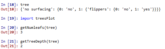
我们先给出最终的决策树图来验证上述结果的正确性

可以看出树的深度确实是有两层，叶节点的数目是3。接下来我们给出绘制决策树图的关键函数，结果就得到上图中决策树。

def plotMidText(cntrPt,parentPt,txtString):
 xMid = (parentPt[0]-cntrPt[0])/2.0+cntrPt[0]
 yMid = (parentPt[1]-cntrPt[1])/2.0+cntrPt[1]
 createPlot.ax1.text(xMid,yMid,txtString)
 
def plotTree(myTree,parentPt,nodeTxt):
 numLeafs = getNumleafs(myTree)
 depth = getTreeDepth(myTree)
 key_sorted= sorted(myTree.keys())
 firstStr = key_sorted[0]
 cntrPt = (plotTree.xOff+(1.0+float(numLeafs))/2.0/plotTree.totalW,plotTree.yOff)
 plotMidText(cntrPt,parentPt,nodeTxt)
 plotNode(firstStr,cntrPt,parentPt,decisionNode)
 secondDict = myTree[firstStr]
 plotTree.yOff -= 1.0/plotTree.totalD
 for key in secondDict.keys():
  if type(secondDict[key]).__name__ == 'dict':
   plotTree(secondDict[key],cntrPt,str(key))
  else:
   plotTree.xOff+=1.0/plotTree.totalW
   plotNode(secondDict[key],(plotTree.xOff,plotTree.yOff),cntrPt,leafNode)
   plotMidText((plotTree.xOff,plotTree.yOff),cntrPt,str(key))
 plotTree.yOff+=1.0/plotTree.totalD
 
def createPlot(inTree):
 fig = plt.figure(1,facecolor = 'white')
 fig.clf()
 axprops = dict(xticks = [],yticks = [])
 createPlot.ax1 = plt.subplot(111,frameon = False,**axprops)
 plotTree.totalW = float(getNumleafs(inTree))
 plotTree.totalD = float(getTreeDepth(inTree))
 plotTree.xOff = -0.5/ plotTree.totalW; plotTree.yOff = 1.0
 plotTree(inTree,(0.5,1.0),'')
 plt.show()
以上就是本文的全部内容，希望对大家的学习有所帮助