数据可视化发现「吃鸡」秘密

大吉大利，今晚吃鸡~

今天跟朋友玩了几把吃鸡，经历了各种死法，还被嘲笑说论女生吃鸡的100种死法，比如被拳头抡死、跳伞落到房顶边缘摔死 、把吃鸡玩成飞车被车技秀死、被队友用燃烧瓶烧死的。这种游戏对我来说就是一个让我明白原来还有这种死法的游戏。

但是玩归玩，还是得假装一下我沉迷学习，所以今天就用吃鸡比赛的真实数据来看看，如何提高你吃鸡的概率。

那么我们就用Python和R做数据分析来回答以下的灵魂发问。

首先来看下数据：

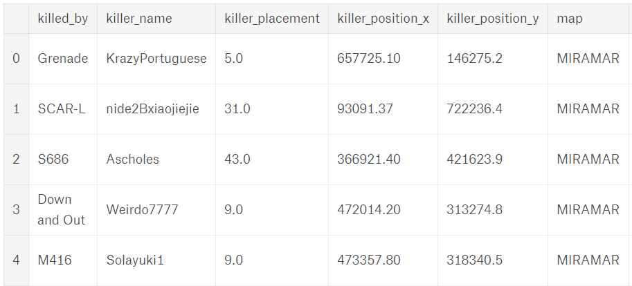
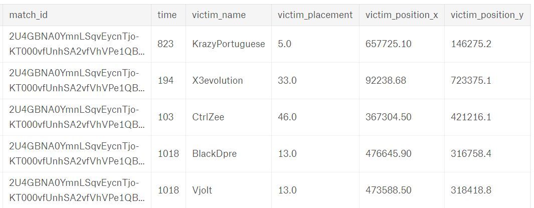
1、跳哪儿危险？

对于我这样一直喜欢苟着的良心玩家，在经历了无数次落地成河的惨痛经历后，我是坚决不会选择跳P城这样楼房密集的城市，穷归穷但保命要紧。

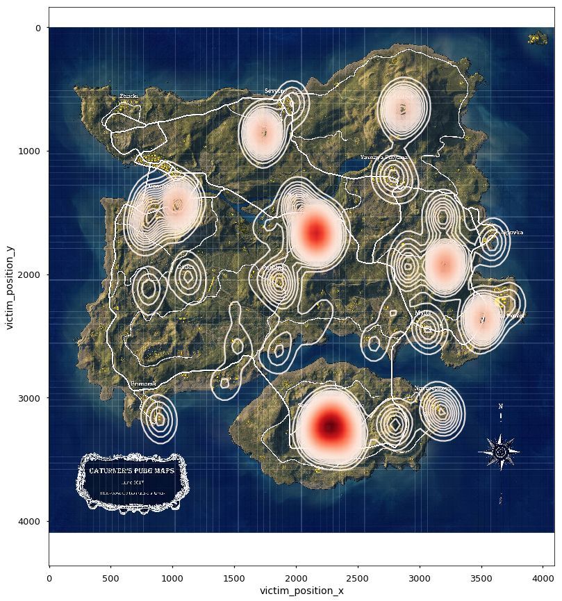
所以我们决定统计一下，到底哪些地方更容易落地成河？

我们筛选出在前100秒死亡的玩家地点进行可视化分析。激情沙漠地图的电站、皮卡多、别墅区、依波城最为危险，火车站、火电厂相对安全。绝地海岛中P城、军事基地、学校、医院、核电站、防空洞都是绝对的危险地带。物质丰富的G港居然相对安全。

1importnumpyasnp

2importmatplotlib.pyplotasplt

3importpandasaspd

4importseabornassns

5fromscipy.misc.pilutilimportimread

6importmatplotlib.cmascm

7

8#导入部分数据

9deaths1 = pd.read_csv("deaths/kill_match_stats_final_0.csv")

10deaths2 = pd.read_csv("deaths/kill_match_stats_final_1.csv")

11

12deaths = pd.concat([deaths1, deaths2])

13

14#打印前5列，理解变量

15print(deaths.head(),'n',len(deaths))

16

17#两种地图

18miramar = deaths[deaths["map"] =="MIRAMAR"]

19erangel = deaths[deaths["map"] =="ERANGEL"]

20

21#开局前100秒死亡热力图

22position_data = ["killer_position_x","killer_position_y","victim_position_x","victim_position_y"]

23forpositioninposition_data:

24miramar[position] = miramar[position].apply(lambdax: x*1000/800000)

25miramar = miramar[miramar[position] !=0]

26

27erangel[position] = erangel[position].apply(lambdax: x*4096/800000)

28erangel = erangel[erangel[position] !=0]

29

30n =50000

31mira_sample = miramar[miramar["time"] <100].sample(n)

32eran_sample = erangel[erangel["time"] <100].sample(n)

33

34# miramar热力图

35bg = imread("miramar.jpg")

36fig, ax = plt.subplots(1,1,figsize=(15,15))

37ax.imshow(bg)

38sns.kdeplot(mira_sample["victim_position_x"], mira_sample["victim_position_y"],n_levels=100, cmap=cm.Reds, alpha=0.9)

39

40# erangel热力图

41bg = imread("erangel.jpg")

42fig, ax = plt.subplots(1,1,figsize=(15,15))

43ax.imshow(bg)

44sns.kdeplot(eran_sample["victim_position_x"], eran_sample["victim_position_y"], n_levels=100,cmap=cm.Reds, alpha=0.9)

2、苟着还是出去干？

我到底是苟在房间里面还是出去和敌人硬拼？

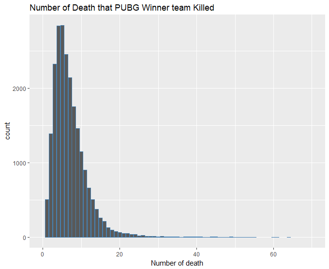
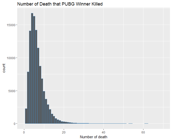
这里因为比赛的规模不一样，这里选取参赛人数大于90的比赛数据，然后筛选出团队team_placement即最后成功吃鸡的团队数据。

1、先计算了吃鸡团队平均击杀敌人的数量，这里剔除了四人模式的比赛数据，因为人数太多的团队会因为数量悬殊平均而变得没意义；

2、所以我们考虑通过分组统计每一组吃鸡中存活到最后的成员击杀敌人的数量，但是这里发现数据统计存活时间变量是按照团队最终存活时间记录的，所以该想法失败；

3、最后统计每个吃鸡团队中击杀人数最多的数量统计，这里剔除了单人模式的数据，因为单人模式的数量就是每组击杀最多的数量。

最后居然发现还有击杀数量达到60的，怀疑是否有开挂。想要吃鸡还是得出去练枪法，光是苟着是不行的。

1library(dplyr)

2library(tidyverse)

3library(data.table)

4library(ggplot2)

5pubg_full <- fread("../agg_match_stats.csv")

6# 吃鸡团队平均击杀敌人的数量

7attach(pubg_full)

8pubg_winner <- pubg_full %>% filter(team_placement==1&party_size<4&game_size>90)

9detach(pubg_full)

10team_killed <- aggregate(pubg_winner$player_kills, by=list(pubg_winner$match_id,pubg_winner$team_id), FUN="mean")

11team_killed$death_num <- ceiling(team_killed$x)

12ggplot(data = team_killed) + geom_bar(mapping = aes(x = death_num, y = ..count..), color="steelblue") +

13xlim(0,70) + labs(title ="Number of Death that PUBG Winner team Killed", x="Number of death")

14

15# 吃鸡团队最后存活的玩家击杀数量

16pubg_winner <- pubg_full %>% filter(pubg_full$team_placement==1) %>% group_by(match_id,team_id)

17attach(pubg_winner)

18team_leader <- aggregate(player_survive_time~player_kills, data = pubg_winner, FUN="max")

19detach(pubg_winner)

20

21# 吃鸡团队中击杀敌人最多的数量

22pubg_winner <- pubg_full %>% filter(pubg_full$team_placement==1&pubg_full$party_size>1)

23attach(pubg_winner)

24team_leader <- aggregate(player_kills, by=list(match_id,team_id), FUN="max")

25detach(pubg_winner)

26ggplot(data = team_leader) + geom_bar(mapping = aes(x = x, y = ..count..), color="steelblue") +

27xlim(0,70) + labs(title ="Number of Death that PUBG Winner Killed", x="Number of death")

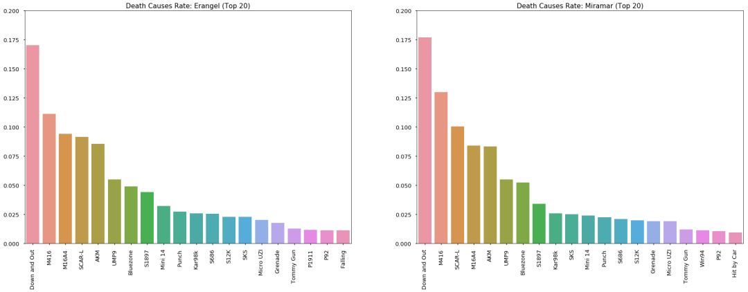
3、哪一种武器干掉的玩家多？

运气好挑到好武器的时候，你是否犹豫选择哪一件？

从图上来看，M416和SCAR是不错的武器，也是相对容易能捡到的武器，大家公认Kar98k是能一枪毙命的好枪，它排名比较靠后的原因也是因为这把枪在比赛比较难得，而且一下击中敌人也是需要实力的，像我这种捡到98k还装上8倍镜但没捂热乎1分钟的玩家是不配得到它的。（捂脸）

1#杀人武器排名

2death_causes = deaths['killed_by'].value_counts()

3

4sns.set_context('talk')

5fig = plt.figure(figsize=(30,10))

6ax = sns.barplot(x=death_causes.index, y=[v / sum(death_causes)forvindeath_causes.values])

7ax.set_title('Rate of Death Causes')

8ax.set_xticklabels(death_causes.index, rotation=90)

9

10#排名前20的武器

11rank =20

12fig = plt.figure(figsize=(20,10))

13ax = sns.barplot(x=death_causes[:rank].index, y=[v / sum(death_causes)forvindeath_causes[:rank].values])

14ax.set_title('Rate of Death Causes')

15ax.set_xticklabels(death_causes.index, rotation=90)

16

17#两个地图分开取

18f, axes = plt.subplots(1,2, figsize=(30,10))

19axes[0].set_title('Death Causes Rate: Erangel (Top {})'.format(rank))

20axes[1].set_title('Death Causes Rate: Miramar (Top {})'.format(rank))

21

22counts_er = erangel['killed_by'].value_counts()

23counts_mr = miramar['killed_by'].value_counts()

24

25sns.barplot(x=counts_er[:rank].index, y=[v / sum(counts_er)forvincounts_er.values][:rank], ax=axes[0] )

26sns.barplot(x=counts_mr[:rank].index, y=[v / sum(counts_mr)forvincounts_mr.values][:rank], ax=axes[1] )

27axes[0].set_ylim((0,0.20))

28axes[0].set_xticklabels(counts_er.index, rotation=90)

29axes[1].set_ylim((0,0.20))

30axes[1].set_xticklabels(counts_mr.index, rotation=90)

31

32#吃鸡和武器的关系

33win = deaths[deaths["killer_placement"] ==1.0]

34win_causes = win['killed_by'].value_counts()

35

36sns.set_context('talk')

37fig = plt.figure(figsize=(20,10))

38ax = sns.barplot(x=win_causes[:20].index, y=[v / sum(win_causes)forvinwin_causes[:20].values])

39ax.set_title('Rate of Death Causes of Win')

40ax.set_xticklabels(win_causes.index, rotation=90)

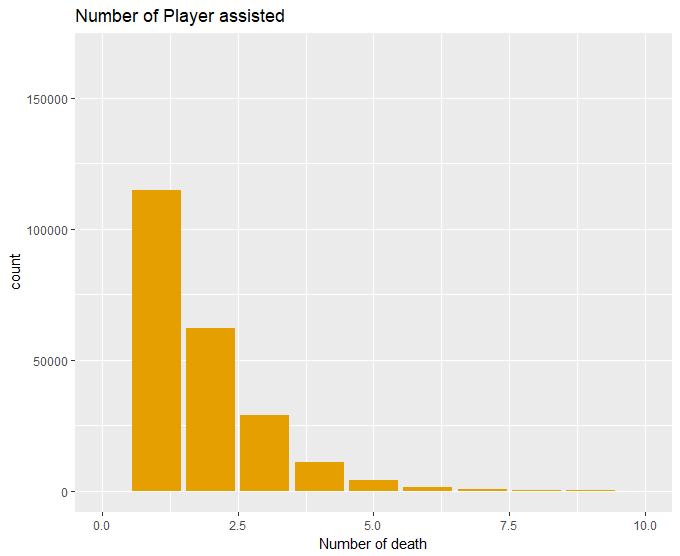
4、队友的助攻是否助我吃鸡？

有时候一不留神就被击倒了，还好我爬得快让队友救我。这里选择成功吃鸡的队伍，最终接受1次帮助的成员所在的团队吃鸡的概率为29%，所以说队友助攻还是很重要的（再不要骂我猪队友了，我也可以选择不救你）。竟然还有让队友救9次的，你也是个人才。（手动滑稽)

1library(dplyr)

2library(tidyverse)

3library(data.table)

4library(ggplot2)

5pubg_full <- fread("E:/aggregate/agg_match_stats_0.csv")

6attach(pubg_full)

7pubg_winner <- pubg_full %>% filter(team_placement==1)

8detach(pubg_full)

9ggplot(data = pubg_winner) + geom_bar(mapping = aes(x = player_assists, y = ..count..), fill="#E69F00") +

10xlim(0,10) + labs(title ="Number of Player assisted", x="Number of death")

11ggplot(data = pubg_winner) + geom_bar(mapping = aes(x = player_assists, y = ..prop..), fill="#56B4E9") +

12xlim(0,10) + labs(title ="Number of Player assisted", x="Number of death")

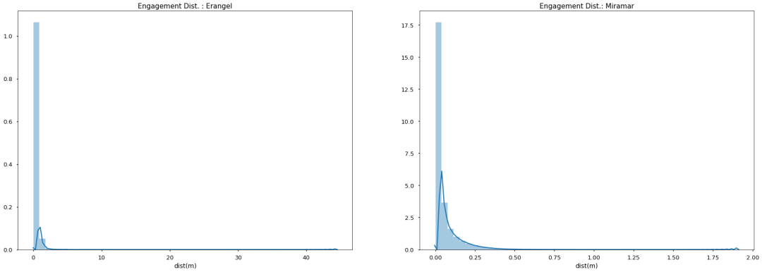
5、敌人离我越近越危险？

对数据中的killer_position和victim_position变量进行欧式距离计算，查看两者的直线距离跟被击倒的分布情况，呈现一个明显的右偏分布，看来还是需要随时观察到附近的敌情，以免到淘汰都不知道敌人在哪儿。

1# python代码：杀人和距离的关系

2importmath

3defget_dist(df):#距离函数

4dist = []

5forrowindf.itertuples():

6subset = (row.killer_position_x - row.victim_position_x)**2+ (row.killer_position_y - row.victim_position_y)**2

7ifsubset >0:

8dist.append(math.sqrt(subset) /100)

9else:

10dist.append(0)

11returndist

12

13df_dist = pd.DataFrame.from_dict({'dist(m)': get_dist(erangel)})

14df_dist.index = erangel.index

15

16erangel_dist = pd.concat([erangel,df_dist], axis=1)

17

18df_dist = pd.DataFrame.from_dict({'dist(m)': get_dist(miramar)})

19df_dist.index = miramar.index

20

21miramar_dist = pd.concat([miramar,df_dist], axis=1)

22

23f, axes = plt.subplots(1,2, figsize=(30,10))

24plot_dist =150

25

26axes[0].set_title('Engagement Dist. : Erangel')

27axes[1].set_title('Engagement Dist.: Miramar')

28

29plot_dist_er = erangel_dist[erangel_dist['dist(m)'] <= plot_dist]

30plot_dist_mr = miramar_dist[miramar_dist['dist(m)'] <= plot_dist]

31

32sns.distplot(plot_dist_er['dist(m)'], ax=axes[0])

33sns.distplot(plot_dist_mr['dist(m)'], ax=axes[1])

6、团队人越多我活得越久？

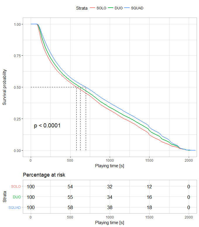
对数据中的party_size变量进行生存分析，可以看到在同一生存率下，四人团队的生存时间高于两人团队，再是单人模式，所以人多力量大这句话不是没有道理的。

7、乘车是否活得更久？

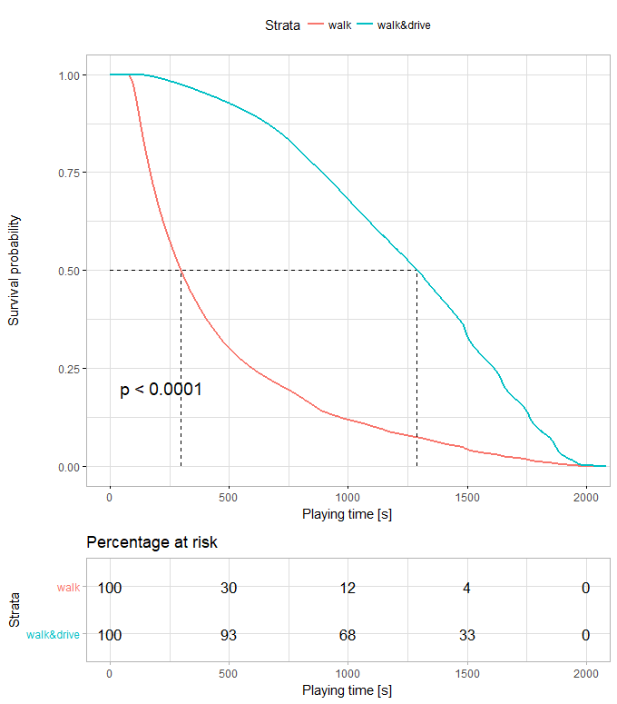
对死因分析中发现，也有不少玩家死于Bluezone，大家天真的以为捡绷带就能跑毒。对数据中的player_dist_ride变量进行生存分析，可以看到在同一生存率下，有开车经历的玩家生存时间高于只走路的玩家，光靠腿你是跑不过毒的。

8、小岛上人越多我活得更久？

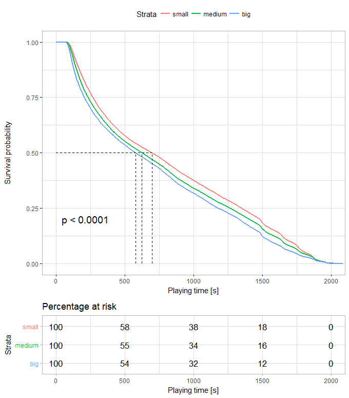
对game_size变量进行生存分析发现还是小规模的比赛比较容易存活。

1# R语言代码如下：

2library(magrittr)

3library(dplyr)

4library(survival)

5library(tidyverse)

6library(data.table)

7library(ggplot2)

8library(survminer)

9pubg_full <- fread("../agg_match_stats.csv")

10# 数据预处理，将连续变量划为分类变量

11pubg_sub <- pubg_full %>%

12filter(player_survive_time<2100) %>%

13mutate(drive = ifelse(player_dist_ride>0,1,0)) %>%

14mutate(size = ifelse(game_size<33,1,ifelse(game_size>=33&game_size<66,2,3)))

15# 创建生存对象

16surv_object <- Surv(time = pubg_sub$player_survive_time)

17fit1 <- survfit(surv_object~party_size,data = pubg_sub)

18# 可视化生存率

19ggsurvplot(fit1, data = pubg_sub, pval =TRUE, xlab="Playing time [s]", surv.median.line="hv",

20legend.labs=c("SOLO","DUO","SQUAD"), ggtheme = theme_light(),risk.table="percentage")

21fit2 <- survfit(surv_object~drive,data=pubg_sub)

22ggsurvplot(fit2, data = pubg_sub, pval =TRUE, xlab="Playing time [s]", surv.median.line="hv",

23legend.labs=c("walk","walk&drive"), ggtheme = theme_light(),risk.table="percentage")

24fit3 <- survfit(surv_object~size,data=pubg_sub)

25ggsurvplot(fit3, data = pubg_sub, pval =TRUE, xlab="Playing time [s]", surv.median.line="hv",

26legend.labs=c("small","medium","big"), ggtheme = theme_light(),risk.table="percentage")

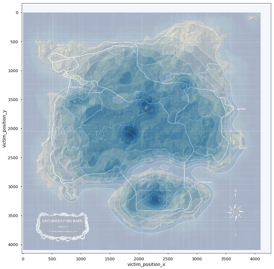
9、最后毒圈有可能出现的地点？

面对有本事能苟到最后的我，怎么样预测最后的毒圈出现在什么位置。

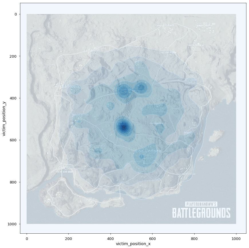
从表agg_match_stats数据找出排名第一的队伍，然后按照match_id分组，找出分组数据里面player_survive_time最大的值，然后据此匹配表格kill_match_stats_final里面的数据，这些数据里面取第二名死亡的位置，作图发现激情沙漠的毒圈明显更集中一些，大概率出现在皮卡多、圣马丁和别墅区。绝地海岛的就比较随机了，但是还是能看出军事基地和山脉的地方更有可能是最后的毒圈。

1#最后毒圈位置

2import matplotlib.pyplot as plt

3import pandas as pd

4import seaborn as sns

5from scipy.misc.pilutil import imread

6import matplotlib.cm as cm

7

8#导入部分数据

9deaths = pd.read_csv("deaths/kill_match_stats_final_0.csv")

10#导入aggregate数据

11aggregate = pd.read_csv("aggregate/agg_match_stats_0.csv")

12print(aggregate.head())

13#找出最后三人死亡的位置

14

15team_win = aggregate[aggregate["team_placement"]==1]#排名第一的队伍

16#找出每次比赛第一名队伍活的最久的那个player

17grouped = team_win.groupby('match_id').apply(lambda t: t[t.player_survive_time==t.player_survive_time.max()])

18

19deaths_solo = deaths[deaths['match_id'].isin(grouped['match_id'].values)]

20deaths_solo_er = deaths_solo[deaths_solo['map'] =='ERANGEL']

21deaths_solo_mr = deaths_solo[deaths_solo['map'] =='MIRAMAR']

22

23df_second_er = deaths_solo_er[(deaths_solo_er['victim_placement'] ==2)].dropna()

24df_second_mr = deaths_solo_mr[(deaths_solo_mr['victim_placement'] ==2)].dropna()

25print (df_second_er)

26

27position_data = ["killer_position_x","killer_position_y","victim_position_x","victim_position_y"]

28forpositioninposition_data:

29df_second_mr[position] = df_second_mr[position].apply(lambda x: x*1000/800000)

30df_second_mr = df_second_mr[df_second_mr[position] !=0]

31

32df_second_er[position] = df_second_er[position].apply(lambda x: x*4096/800000)

33df_second_er = df_second_er[df_second_er[position] !=0]

34

35df_second_er=df_second_er

36# erangel热力图

37sns.set_context('talk')

38bg = imread("erangel.jpg")

39fig, ax = plt.subplots(1,1,figsize=(15,15))

40ax.imshow(bg)

41sns.kdeplot(df_second_er["victim_position_x"], df_second_er["victim_position_y"], cmap=cm.Blues, alpha=0.7,shade=True)

42

43# miramar热力图

44bg = imread("miramar.jpg")

45fig, ax = plt.subplots(1,1,figsize=(15,15))

46ax.imshow(bg)

47sns.kdeplot(df_second_mr["victim_position_x"], df_second_mr["victim_position_y"], cmap=cm.Blues,alpha=0.8,shade=True)

最后祝大家：