小姐姐带你一起学:如何用Python实现7种机器学习算法(附代码)
Python 被称为是最接近 AI 的语言。最近一位名叫Anna-Lena Popkes的小姐姐在GitHub上分享了自己如何使用Python(3.6及以上版本)实现7种机器学习算法的笔记,并附有完整代码。所有这些算法的实现都没有使用其他机器学习库。这份笔记可以帮大家对算法以及其底层结构有个基本的了解,但并不是提供最有效的实现。
小姐姐她是德国波恩大学计算机科学专业的研究生,主要关注机器学习和神经网络。

七种算法包括:
▌1. 线性回归算法
在线性回归中,我们想要建立一个模型,来拟合一个因变量 y 与一个或多个独立自变量(预测变量) x 之间的关系。
给定:
线性回归模型可以使用以下方法进行训练
a) 梯度下降法
b) 正态方程(封闭形式解):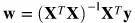
其中 X 是一个矩阵,其形式为 ,包含所有训练样本的维度信息。
而正态方程需要计算 的转置。这个操作的计算复杂度介于
 )和
)和 之间,而这取决于所选择的实现方法。因此,如果训练集中数据的特征数量很大,那么使用正态方程训练的过程将变得非常缓慢。
线性回归模型的训练过程有不同的步骤。首先(在步骤 0 中),模型的参数将被初始化。在达到指定训练次数或参数收敛前,重复以下其他步骤。
第 0 步:
用0 (或小的随机值)来初始化权重向量和偏置量,或者直接使用正态方程计算模型参数
第 1 步(只有在使用梯度下降法训练时需要):
计算输入的特征与权重值的线性组合,这可以通过矢量化和矢量传播来对所有训练样本进行处理: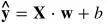
其中 X 是所有训练样本的维度矩阵,其形式为 ;· 表示点积。
第 2 步(只有在使用梯度下降法训练时需要):
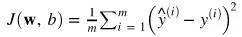
用均方误差计算训练集上的损失:
第 3 步(只有在使用梯度下降法训练时需要):
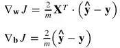
对每个参数,计算其对损失函数的偏导数:
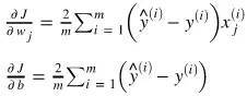
所有偏导数的梯度计算如下:
第 4 步(只有在使用梯度下降法训练时需要):
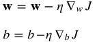
更新权重向量和偏置量:
其中, 表示学习率。
In [4]:
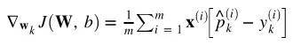
import numpy as npimport matplotlib.pyplot as pltfrom sklearn.model_selection import train_test_splitnp.random.seed(123)
数据集
In [5]:
# We will use a simple training setX = 2 * np.random.rand(500, 1)y = 5 + 3 * X + np.random.randn(500, 1)fig = plt.figure(figsize=(8,6))plt.scatter(X, y)plt.title("Dataset")plt.xlabel("First feature")plt.ylabel("Second feature")plt.show()

In [6]:
# Split the data into a training and test setX_train, X_test, y_train, y_test = train_test_split(X, y)print(f'Shape X_train: {X_train.shape}')print(f'Shape y_train: {y_train.shape}')print(f'Shape X_test: {X_test.shape}')print(f'Shape y_test: {y_test.shape}')
Shape X_train: (375, 1)Shape y_train: (375, 1)Shape X_test: (125, 1)Shape y_test: (125, 1)
线性回归分类
In [23]:
class LinearRegression: def __init__(self): pass def train_gradient_descent(self, X, y, learning_rate=0.01, n_iters=100): """ Trains a linear regression model using gradient descent """ # Step 0: Initialize the parameters n_samples, n_features = X.shape self.weights = np.zeros(shape=(n_features,1)) self.bias = 0 costs = [] for i in range(n_iters): # Step 1: Compute a linear combination of the input features and weights y_predict = np.dot(X, self.weights) + self.bias # Step 2: Compute cost over training set cost = (1 / n_samples) * np.sum((y_predict - y)**2) costs.append(cost) if i % 100 == 0: print(f"Cost at iteration {i}: {cost}") # Step 3: Compute the gradients dJ_dw = (2 / n_samples) * np.dot(X.T, (y_predict - y)) dJ_db = (2 / n_samples) * np.sum((y_predict - y)) # Step 4: Update the parameters self.weights = self.weights - learning_rate * dJ_dw self.bias = self.bias - learning_rate * dJ_db return self.weights, self.bias, costs def train_normal_equation(self, X, y): """ Trains a linear regression model using the normal equation """ self.weights = np.dot(np.dot(np.linalg.inv(np.dot(X.T, X)), X.T), y) self.bias = 0 return self.weights, self.bias def predict(self, X): return np.dot(X, self.weights) + self.bias
使用梯度下降进行训练
In [24]:
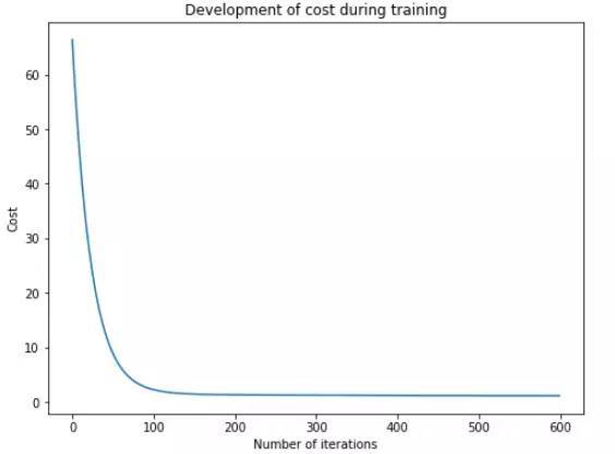
regressor = LinearRegression()w_trained, b_trained, costs = regressor.train_gradient_descent(X_train, y_train, learning_rate=0.005, n_iters=600)fig = plt.figure(figsize=(8,6))plt.plot(np.arange(n_iters), costs)plt.title("Development of cost during training")plt.xlabel("Number of iterations")plt.ylabel("Cost")plt.show()
Cost at iteration 0: 66.45256981003433Cost at iteration 100: 2.2084346146095934Cost at iteration 200: 1.2797812854182806Cost at iteration 300: 1.2042189195356685Cost at iteration 400: 1.1564867816573Cost at iteration 500: 1.121391041394467
测试(梯度下降模型)
In [28]:
n_samples, _ = X_train.shapen_samples_test, _ = X_test.shapey_p_train = regressor.predict(X_train)y_p_test = regressor.predict(X_test)error_train = (1 / n_samples) * np.sum((y_p_train - y_train) ** 2)error_test = (1 / n_samples_test) * np.sum((y_p_test - y_test) ** 2)print(f"Error on training set: {np.round(error_train, 4)}")print(f"Error on test set: {np.round(error_test)}")
Error on training set: 1.0955
Error on test set: 1.0
使用正规方程(normal equation)训练
# To compute the parameters using the normal equation, we add a bias value of 1 to each input exampleX_b_train = np.c_[np.ones((n_samples)), X_train]X_b_test = np.c_[np.ones((n_samples_test)), X_test]reg_normal = LinearRegression()w_trained = reg_normal.train_normal_equation(X_b_train, y_train)
测试(正规方程模型)
y_p_train = reg_normal.predict(X_b_train)y_p_test = reg_normal.predict(X_b_test)error_train = (1 / n_samples) * np.sum((y_p_train - y_train) ** 2)error_test = (1 / n_samples_test) * np.sum((y_p_test - y_test) ** 2)print(f"Error on training set: {np.round(error_train, 4)}")print(f"Error on test set: {np.round(error_test, 4)}")
Error on training set: 1.0228
Error on test set: 1.0432
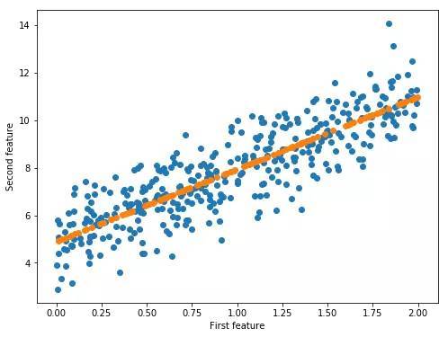
可视化测试预测
# Plot the test predictionsfig = plt.figure(figsize=(8,6))plt.scatter(X_train, y_train)plt.scatter(X_test, y_p_test)plt.xlabel("First feature")plt.ylabel("Second feature")plt.show()
▌2. Logistic 回归算法
在 Logistic 回归中,我们试图对给定输入特征的线性组合进行建模,来得到其二元变量的输出结果。例如,我们可以尝试使用竞选候选人花费的金钱和时间信息来预测选举的结果(胜或负)。Logistic 回归算法的工作原理如下。
给定:
Logistic 回归模型可以理解为一个非常简单的神经网络:
与线性回归不同,Logistic 回归没有封闭解。但由于损失函数是凸函数,因此我们可以使用梯度下降法来训练模型。事实上,在保证学习速率足够小且使用足够的训练迭代步数的前提下,梯度下降法(或任何其他优化算法)可以是能够找到全局最小值。
训练 Logistic 回归模型有不同的步骤。首先(在步骤 0 中),模型的参数将被初始化。在达到指定训练次数或参数收敛前,重复以下其他步骤。
第 0 步:用 0 (或小的随机值)来初始化权重向量和偏置值
第 1 步:计算输入的特征与权重值的线性组合,这可以通过矢量化和矢量传播来对所有训练样本进行处理: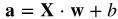
其中 X 是所有训练样本的维度矩阵,其形式为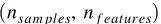 ;·表示点积。
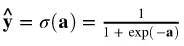
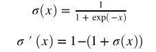
第 2 步:用 sigmoid 函数作为激活函数,其返回值介于0到1之间:
第 3 步:计算整个训练集的损失值。
我们希望模型得到的目标值概率落在 0 到 1 之间。因此在训练期间,我们希望调整参数,使得模型较大的输出值对应正标签(真实标签为 1),较小的输出值对应负标签(真实标签为 0 )。这在损失函数中表现为如下形式:

第 4 步:对权重向量和偏置量,计算其对损失函数的梯度。
关于这个导数实现的详细解释,可以参见这里(https://stats.stackexchange.com/questions/278771/how-is-the-cost-function-from-logistic-regression-derivated)。
一般形式如下:

对于偏置量的导数计算,此时 为 1。
为 1。
第 5 步:更新权重和偏置值。
其中,表示学习率。
In [24]:
import numpy as npfrom sklearn.model_selection import train_test_splitfrom sklearn.datasets import make_blobsimport matplotlib.pyplot as pltnp.random.seed(123)% matplotlib inline
数据集
In [25]:
# We will perform logistic regression using a simple toy dataset of two classesX, y_true = make_blobs(n_samples= 1000, centers=2)fig = plt.figure(figsize=(8,6))plt.scatter(X[:,0], X[:,1], c=y_true)plt.title("Dataset")plt.xlabel("First feature")plt.ylabel("Second feature")plt.show()
In [26]:
# Reshape targets to get column vector with shape (n_samples, 1)y_true = y_true[:, np.newaxis]# Split the data into a training and test setX_train, X_test, y_train, y_test = train_test_split(X, y_true)print(f'Shape X_train: {X_train.shape}')print(f'Shape y_train: {y_train.shape}')print(f'Shape X_test: {X_test.shape}')print(f'Shape y_test: {y_test.shape}')
Shape X_train: (750, 2)
Shape y_train: (750, 1)
Shape X_test: (250, 2)
Shape y_test: (250, 1)
Logistic回归分类
In [27]:
class LogisticRegression: def __init__(self): pass def sigmoid(self, a): return 1 / (1 + np.exp(-a)) def train(self, X, y_true, n_iters, learning_rate): """ Trains the logistic regression model on given data X and targets y """ # Step 0: Initialize the parameters n_samples, n_features = X.shape self.weights = np.zeros((n_features, 1)) self.bias = 0 costs = [] for i in range(n_iters): # Step 1 and 2: Compute a linear combination of the input features and weights, # apply the sigmoid activation function y_predict = self.sigmoid(np.dot(X, self.weights) + self.bias) # Step 3: Compute the cost over the whole training set. cost = (- 1 / n_samples) * np.sum(y_true * np.log(y_predict) + (1 - y_true) * (np.log(1 - y_predict))) # Step 4: Compute the gradients dw = (1 / n_samples) * np.dot(X.T, (y_predict - y_true)) db = (1 / n_samples) * np.sum(y_predict - y_true) # Step 5: Update the parameters self.weights = self.weights - learning_rate * dw self.bias = self.bias - learning_rate * db costs.append(cost) if i % 100 == 0: print(f"Cost after iteration {i}: {cost}") return self.weights, self.bias, costs def predict(self, X): """ Predicts binary labels for a set of examples X. """ y_predict = self.sigmoid(np.dot(X, self.weights) + self.bias) y_predict_labels = [1 if elem > 0.5 else 0 for elem in y_predict] return np.array(y_predict_labels)[:, np.newaxis]
初始化并训练模型
In [29]:
regressor = LogisticRegression()w_trained, b_trained, costs = regressor.train(X_train, y_train, n_iters=600, learning_rate=0.009)fig = plt.figure(figsize=(8,6))plt.plot(np.arange(600), costs)plt.title("Development of cost over training")plt.xlabel("Number of iterations")plt.ylabel("Cost")plt.show()
Cost after iteration 0: 0.6931471805599453
Cost after iteration 100: 0.046514002935609956
Cost after iteration 200: 0.02405337743999163
Cost after iteration 300: 0.016354408151412207
Cost after iteration 400: 0.012445770521974634
Cost after iteration 500: 0.010073981792906512

测试模型
In [31]:
y_p_train = regressor.predict(X_train)y_p_test = regressor.predict(X_test)print(f"train accuracy: {100 - np.mean(np.abs(y_p_train - y_train)) * 100}%")print(f"test accuracy: {100 - np.mean(np.abs(y_p_test - y_test))}%")
train accuracy: 100.0%
test accuracy: 100.0%
▌3. 感知器算法
感知器是一种简单的监督式的机器学习算法,也是最早的神经网络体系结构之一。它由 Rosenblatt 在 20 世纪 50 年代末提出。感知器是一种二元的线性分类器,其使用 d- 维超平面来将一组训练样本( d- 维输入向量)映射成二进制输出值。它的原理如下:
给定:
感知器可以理解为一个非常简单的神经网络:
感知器的训练可以使用梯度下降法,训练算法有不同的步骤。首先(在步骤0中),模型的参数将被初始化。在达到指定训练次数或参数收敛前,重复以下其他步骤。
第 0 步:用 0 (或小的随机值)来初始化权重向量和偏置值
第 1 步:计算输入的特征与权重值的线性组合,这可以通过矢量化和矢量传播法则来对所有训练样本进行处理:
其中 X 是所有训练示例的维度矩阵,其形式为;·表示点积。
第 2 步:用 Heaviside step 函数作为激活函数,其返回一个二进制值:
第 3 步:使用感知器的学习规则来计算权重向量和偏置量的更新值。

其中,表示学习率。
第 4 步:更新权重向量和偏置量。
In [1]:
import numpy as npimport matplotlib.pyplot as pltfrom sklearn.datasets import make_blobsfrom sklearn.model_selection import train_test_splitnp.random.seed(123)% matplotlib inline
数据集
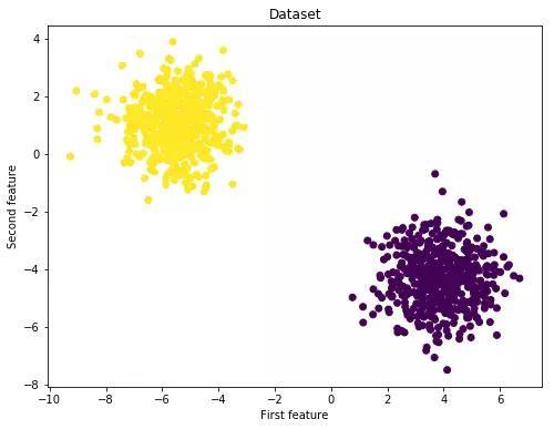
In [2]:
X, y = make_blobs(n_samples=1000, centers=2)fig = plt.figure(figsize=(8,6))plt.scatter(X[:,0], X[:,1], c=y)plt.title("Dataset")plt.xlabel("First feature")plt.ylabel("Second feature")plt.show()
In [3]:
y_true = y[:, np.newaxis]X_train, X_test, y_train, y_test = train_test_split(X, y_true)print(f'Shape X_train: {X_train.shape}')print(f'Shape y_train: {y_train.shape})')print(f'Shape X_test: {X_test.shape}')print(f'Shape y_test: {y_test.shape}')
Shape X_train: (750, 2)
Shape y_train: (750, 1))
Shape X_test: (250, 2)
Shape y_test: (250, 1)
感知器分类
In [6]:
class Perceptron(): def __init__(self): pass def train(self, X, y, learning_rate=0.05, n_iters=100): n_samples, n_features = X.shape # Step 0: Initialize the parameters self.weights = np.zeros((n_features,1)) self.bias = 0 for i in range(n_iters): # Step 1: Compute the activation a = np.dot(X, self.weights) + self.bias # Step 2: Compute the output y_predict = self.step_function(a) # Step 3: Compute weight updates delta_w = learning_rate * np.dot(X.T, (y - y_predict)) delta_b = learning_rate * np.sum(y - y_predict) # Step 4: Update the parameters self.weights += delta_w self.bias += delta_b return self.weights, self.bias def step_function(self, x): return np.array([1 if elem >= 0 else 0 for elem in x])[:, np.newaxis] def predict(self, X): a = np.dot(X, self.weights) + self.bias return self.step_function(a)
初始化并训练模型
In [7]:
p = Perceptron()w_trained, b_trained = p.train(X_train, y_train,learning_rate=0.05, n_iters=500)
测试
In [10]:
y_p_train = p.predict(X_train)y_p_test = p.predict(X_test)print(f"training accuracy: {100 - np.mean(np.abs(y_p_train - y_train)) * 100}%")print(f"test accuracy: {100 - np.mean(np.abs(y_p_test - y_test)) * 100}%")
training accuracy: 100.0%
test accuracy: 100.0%
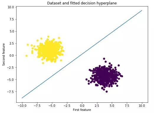
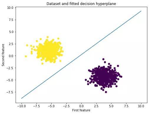
可视化决策边界
In [13]:
def plot_hyperplane(X, y, weights, bias): """ Plots the dataset and the estimated decision hyperplane """ slope = - weights[0]/weights[1] intercept = - bias/weights[1] x_hyperplane = np.linspace(-10,10,10) y_hyperplane = slope * x_hyperplane + intercept fig = plt.figure(figsize=(8,6)) plt.scatter(X[:,0], X[:,1], c=y) plt.plot(x_hyperplane, y_hyperplane, '-') plt.title("Dataset and fitted decision hyperplane") plt.xlabel("First feature") plt.ylabel("Second feature") plt.show()
In [14]:
plot_hyperplane(X, y, w_trained, b_trained)
▌4. K 最近邻算法
k-nn 算法是一种简单的监督式的机器学习算法,可以用于解决分类和回归问题。这是一个基于实例的算法,并不是估算模型,而是将所有训练样本存储在内存中,并使用相似性度量进行预测。
给定一个输入示例,k-nn 算法将从内存中检索 k 个最相似的实例。相似性是根据距离来定义的,也就是说,与输入示例之间距离最小(欧几里得距离)的训练样本被认为是最相似的样本。
输入示例的目标值计算如下:
分类问题:
a) 不加权:输出 k 个最近邻中最常见的分类
b) 加权:将每个分类值的k个最近邻的权重相加,输出权重最高的分类
回归问题:
a) 不加权:输出k个最近邻值的平均值
b) 加权:对于所有分类值,将分类值加权求和并将结果除以所有权重的总和
加权版本的 k-nn 算法是改进版本,其中每个近邻的贡献值根据其与查询点之间的距离进行加权。下面,我们在 sklearn 用 k-nn 算法的原始版本实现数字数据集的分类。
In [1]:
import numpy as npimport matplotlib.pyplot as pltfrom sklearn.datasets import load_digitsfrom sklearn.model_selection import train_test_splitnp.random.seed(123)% matplotlib inline
数据集
In [2]:
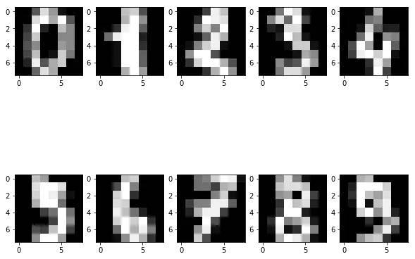
# We will use the digits dataset as an example. It consists of the 1797 images of hand-written digits. Each digit is# represented by a 64-dimensional vector of pixel values.digits = load_digits()X, y = digits.data, digits.targetX_train, X_test, y_train, y_test = train_test_split(X, y)print(f'X_train shape: {X_train.shape}')print(f'y_train shape: {y_train.shape}')print(f'X_test shape: {X_test.shape}')print(f'y_test shape: {y_test.shape}')# Example digitsfig = plt.figure(figsize=(10,8))for i in range(10): ax = fig.add_subplot(2, 5, i+1) plt.imshow(X[i].reshape((8,8)), cmap='gray')
X_train shape: (1347, 64)
y_train shape: (1347,)
X_test shape: (450, 64)
y_test shape: (450,)
K 最邻近类别
In [3]:
class kNN(): def __init__(self): pass def fit(self, X, y): self.data = X self.targets = y def euclidean_distance(self, X): """ Computes the euclidean distance between the training data and a new input example or matrix of input examples X """ # input: single data point if X.ndim == 1: l2 = np.sqrt(np.sum((self.data - X)**2, axis=1)) # input: matrix of data points if X.ndim == 2: n_samples, _ = X.shape l2 = [np.sqrt(np.sum((self.data - X[i])**2, axis=1)) for i in range(n_samples)] return np.array(l2) def predict(self, X, k=1): """ Predicts the classification for an input example or matrix of input examples X """ # step 1: compute distance between input and training data dists = self.euclidean_distance(X) # step 2: find the k nearest neighbors and their classifications if X.ndim == 1: if k == 1: nn = np.argmin(dists) return self.targets[nn] else: knn = np.argsort(dists)[:k] y_knn = self.targets[knn] max_vote = max(y_knn, key=list(y_knn).count) return max_vote if X.ndim == 2: knn = np.argsort(dists)[:, :k] y_knn = self.targets[knn] if k == 1: return y_knn.T else: n_samples, _ = X.shape max_votes = [max(y_knn[i], key=list(y_knn[i]).count) for i in range(n_samples)] return max_votes
初始化并训练模型
In [11]:
knn = kNN()knn.fit(X_train, y_train)print("Testing one datapoint, k=1")print(f"Predicted label: {knn.predict(X_test[0], k=1)}")print(f"True label: {y_test[0]}")print()print("Testing one datapoint, k=5")print(f"Predicted label: {knn.predict(X_test[20], k=5)}")print(f"True label: {y_test[20]}")print()print("Testing 10 datapoint, k=1")print(f"Predicted labels: {knn.predict(X_test[5:15], k=1)}")print(f"True labels: {y_test[5:15]}")print()print("Testing 10 datapoint, k=4")print(f"Predicted labels: {knn.predict(X_test[5:15], k=4)}")print(f"True labels: {y_test[5:15]}")print()
Testing one datapoint, k=1
Predicted label: 3
True label: 3
Testing one datapoint, k=5
Predicted label: 9
True label: 9
Testing 10 datapoint, k=1
Predicted labels: [[3 1 0 7 4 0 0 5 1 6]]
True labels: [3 1 0 7 4 0 0 5 1 6]
Testing 10 datapoint, k=4
Predicted labels: [3, 1, 0, 7, 4, 0, 0, 5, 1, 6]
True labels: [3 1 0 7 4 0 0 5 1 6]
测试集精度
In [12]:
# Compute accuracy on test sety_p_test1 = knn.predict(X_test, k=1)test_acc1= np.sum(y_p_test1[0] == y_test)/len(y_p_test1[0]) * 100print(f"Test accuracy with k = 1: {format(test_acc1)}")y_p_test8 = knn.predict(X_test, k=5)test_acc8= np.sum(y_p_test8 == y_test)/len(y_p_test8) * 100print(f"Test accuracy with k = 8: {format(test_acc8)}")
Test accuracy with k = 1: 97.77777777777777
Test accuracy with k = 8: 97.55555555555556
▌5. K均值聚类算法
K-Means 是一种非常简单的聚类算法(聚类算法都属于无监督学习)。给定固定数量的聚类和输入数据集,该算法试图将数据划分为聚类,使得聚类内部具有较高的相似性,聚类与聚类之间具有较低的相似性。
算法原理
1. 初始化聚类中心,或者在输入数据范围内随机选择,或者使用一些现有的训练样本(推荐)
2. 直到收敛
目标函数
聚类算法的目标函数试图找到聚类中心,以便数据将划分到相应的聚类中,并使得数据与其最接近的聚类中心之间的距离尽可能小。
给定一组数据X1,...,Xn和一个正数k,找到k个聚类中心C1,...,Ck并最小化目标函数:
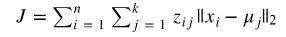
这里:
K-Means 算法的缺点:
In [21]:
import numpy as npimport matplotlib.pyplot as pltimport randomfrom sklearn.datasets import make_blobsnp.random.seed(123)% matplotlib inline
数据集
In [22]:
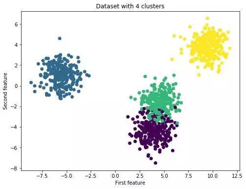
X, y = make_blobs(centers=4, n_samples=1000)print(f'Shape of dataset: {X.shape}')fig = plt.figure(figsize=(8,6))plt.scatter(X[:,0], X[:,1], c=y)plt.title("Dataset with 4 clusters")plt.xlabel("First feature")plt.ylabel("Second feature")plt.show()
Shape of dataset: (1000, 2)
K均值分类
In [23]:
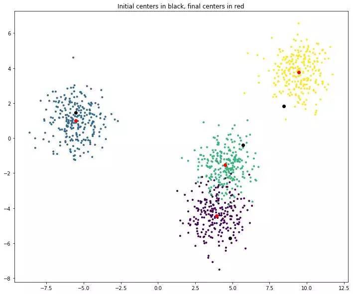
class KMeans(): def __init__(self, n_clusters=4): self.k = n_clusters def fit(self, data): """ Fits the k-means model to the given dataset """ n_samples, _ = data.shape # initialize cluster centers self.centers = np.array(random.sample(list(data), self.k)) self.initial_centers = np.copy(self.centers) # We will keep track of whether the assignment of data points # to the clusters has changed. If it stops changing, we are # done fitting the model old_assigns = None n_iters = 0 while True: new_assigns = [self.classify(datapoint) for datapoint in data] if new_assigns == old_assigns: print(f"Training finished after {n_iters} iterations!") return old_assigns = new_assigns n_iters += 1 # recalculate centers for id_ in range(self.k): points_idx = np.where(np.array(new_assigns) == id_) datapoints = data[points_idx] self.centers[id_] = datapoints.mean(axis=0) def l2_distance(self, datapoint): dists = np.sqrt(np.sum((self.centers - datapoint)**2, axis=1)) return dists def classify(self, datapoint): """ Given a datapoint, compute the cluster closest to the datapoint. Return the cluster ID of that cluster. """ dists = self.l2_distance(datapoint) return np.argmin(dists) def plot_clusters(self, data): plt.figure(figsize=(12,10)) plt.title("Initial centers in black, final centers in red") plt.scatter(data[:, 0], data[:, 1], marker='.', c=y) plt.scatter(self.centers[:, 0], self.centers[:,1], c='r') plt.scatter(self.initial_centers[:, 0], self.initial_centers[:,1], c='k') plt.show()
初始化并调整模型
kmeans = KMeans(n_clusters=4)kmeans.fit(X)
Training finished after 4 iterations!
描绘初始和最终的聚类中心
kmeans.plot_clusters(X)
▌6. 简单的神经网络
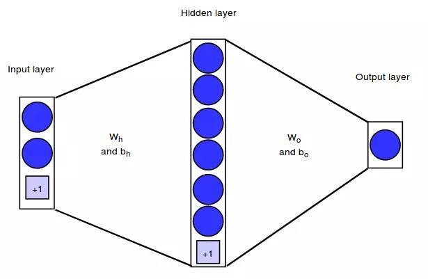
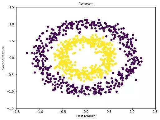
在这一章节里,我们将实现一个简单的神经网络架构,将 2 维的输入向量映射成二进制输出值。我们的神经网络有 2 个输入神经元,含 6 个隐藏神经元隐藏层及 1 个输出神经元。
我们将通过层之间的权重矩阵来表示神经网络结构。在下面的例子中,输入层和隐藏层之间的权重矩阵将被表示为 ,隐藏层和输出层之间的权重矩阵为
 。除了连接神经元的权重向量外,每个隐藏和输出的神经元都会有一个大小为 1 的偏置量。
我们的训练集由 m = 750 个样本组成。因此,我们的矩阵维度如下:
我们使用与 Logistic 回归算法相同的损失函数:
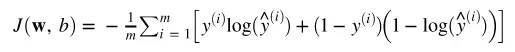
对于多类别的分类任务,我们将使用这个函数的通用形式作为损失函数,称之为分类交叉熵函数。
训练
我们将用梯度下降法来训练我们的神经网络,并通过反向传播法来计算所需的偏导数。训练过程主要有以下几个步骤:
1. 初始化参数(即权重量和偏差量)
2. 重复以下过程,直到收敛:
前向传播过程
首先,我们计算网络中每个单元的激活值和输出值。为了加速这个过程的实现,我们不会单独为每个输入样本执行此操作,而是通过矢量化对所有样本一次性进行处理。其中:
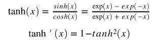
隐层神经元将使用 tanh 函数作为其激活函数:
输出层神经元将使用 sigmoid 函数作为激活函数:
激活值和输出值计算如下(·表示点乘):

反向传播过程
为了计算权重向量的更新值,我们需要计算每个神经元对损失函数的偏导数。这里不会给出这些公式的推导,你会在其他网站上找到很多更好的解释(https://mattmazur.com/2015/03/17/a-step-by-step-backpropagation-example/)。
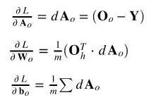
对于输出神经元,梯度计算如下(矩阵符号):
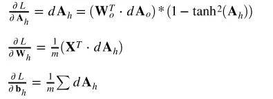
对于输入和隐层的权重矩阵,梯度计算如下:
权重更新

In [3]:
import numpy as npimport pandas as pdimport matplotlib.pyplot as pltfrom sklearn.datasets import make_circlesfrom sklearn.model_selection import train_test_splitnp.random.seed(123)% matplotlib inline
数据集
In [4]:
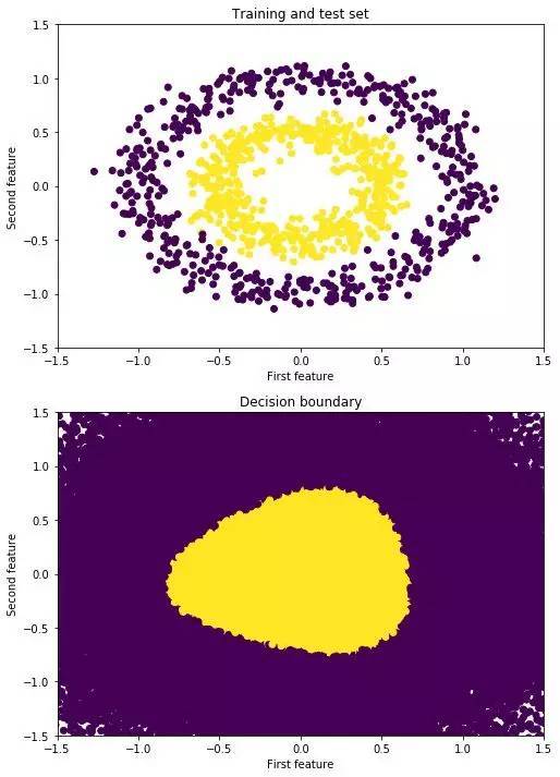
X, y = make_circles(n_samples=1000, factor=0.5, noise=.1)fig = plt.figure(figsize=(8,6))plt.scatter(X[:,0], X[:,1], c=y)plt.xlim([-1.5, 1.5])plt.ylim([-1.5, 1.5])plt.title("Dataset")plt.xlabel("First feature")plt.ylabel("Second feature")plt.show()
In [5]:
# reshape targets to get column vector with shape (n_samples, 1)y_true = y[:, np.newaxis]# Split the data into a training and test setX_train, X_test, y_train, y_test = train_test_split(X, y_true)print(f'Shape X_train: {X_train.shape}')print(f'Shape y_train: {y_train.shape}')print(f'Shape X_test: {X_test.shape}')print(f'Shape y_test: {y_test.shape}')
Shape X_train: (750, 2)
Shape y_train: (750, 1)
Shape X_test: (250, 2)
Shape y_test: (250, 1)
Neural Network Class
以下部分实现受益于吴恩达的课程
https://www.coursera.org/learn/neural-networks-deep-learning
class NeuralNet(): def __init__(self, n_inputs, n_outputs, n_hidden): self.n_inputs = n_inputs self.n_outputs = n_outputs self.hidden = n_hidden # Initialize weight matrices and bias vectors self.W_h = np.random.randn(self.n_inputs, self.hidden) self.b_h = np.zeros((1, self.hidden)) self.W_o = np.random.randn(self.hidden, self.n_outputs) self.b_o = np.zeros((1, self.n_outputs)) def sigmoid(self, a): return 1 / (1 + np.exp(-a)) def forward_pass(self, X): """ Propagates the given input X forward through the net. Returns: A_h: matrix with activations of all hidden neurons for all input examples O_h: matrix with outputs of all hidden neurons for all input examples A_o: matrix with activations of all output neurons for all input examples O_o: matrix with outputs of all output neurons for all input examples """ # Compute activations and outputs of hidden units A_h = np.dot(X, self.W_h) + self.b_h O_h = np.tanh(A_h) # Compute activations and outputs of output units A_o = np.dot(O_h, self.W_o) + self.b_o O_o = self.sigmoid(A_o) outputs = { "A_h": A_h, "A_o": A_o, "O_h": O_h, "O_o": O_o, } return outputs def cost(self, y_true, y_predict, n_samples): """ Computes and returns the cost over all examples """ # same cost function as in logistic regression cost = (- 1 / n_samples) * np.sum(y_true * np.log(y_predict) + (1 - y_true) * (np.log(1 - y_predict))) cost = np.squeeze(cost) assert isinstance(cost, float) return cost def backward_pass(self, X, Y, n_samples, outputs): """ Propagates the errors backward through the net. Returns: dW_h: partial derivatives of loss function w.r.t hidden weights db_h: partial derivatives of loss function w.r.t hidden bias dW_o: partial derivatives of loss function w.r.t output weights db_o: partial derivatives of loss function w.r.t output bias """ dA_o = (outputs["O_o"] - Y) dW_o = (1 / n_samples) * np.dot(outputs["O_h"].T, dA_o) db_o = (1 / n_samples) * np.sum(dA_o) dA_h = (np.dot(dA_o, self.W_o.T)) * (1 - np.power(outputs["O_h"], 2)) dW_h = (1 / n_samples) * np.dot(X.T, dA_h) db_h = (1 / n_samples) * np.sum(dA_h) gradients = { "dW_o": dW_o, "db_o": db_o, "dW_h": dW_h, "db_h": db_h, } return gradients def update_weights(self, gradients, eta): """ Updates the model parameters using a fixed learning rate """ self.W_o = self.W_o - eta * gradients["dW_o"] self.W_h = self.W_h - eta * gradients["dW_h"] self.b_o = self.b_o - eta * gradients["db_o"] self.b_h = self.b_h - eta * gradients["db_h"] def train(self, X, y, n_iters=500, eta=0.3): """ Trains the neural net on the given input data """ n_samples, _ = X.shape for i in range(n_iters): outputs = self.forward_pass(X) cost = self.cost(y, outputs["O_o"], n_samples=n_samples) gradients = self.backward_pass(X, y, n_samples, outputs) if i % 100 == 0: print(f'Cost at iteration {i}: {np.round(cost, 4)}') self.update_weights(gradients, eta) def predict(self, X): """ Computes and returns network predictions for given dataset """ outputs = self.forward_pass(X) y_pred = [1 if elem >= 0.5 else 0 for elem in outputs["O_o"]] return np.array(y_pred)[:, np.newaxis]
初始化并训练神经网络
nn = NeuralNet(n_inputs=2, n_hidden=6, n_outputs=1)print("Shape of weight matrices and bias vectors:")print(f'W_h shape: {nn.W_h.shape}')print(f'b_h shape: {nn.b_h.shape}')print(f'W_o shape: {nn.W_o.shape}')print(f'b_o shape: {nn.b_o.shape}')print()print("Training:")nn.train(X_train, y_train, n_iters=2000, eta=0.7)
Shape of weight matrices and bias vectors:
W_h shape: (2, 6)
b_h shape: (1, 6)
W_o shape: (6, 1)
b_o shape: (1, 1)
Training:
Cost at iteration 0: 1.0872
Cost at iteration 100: 0.2723
Cost at iteration 200: 0.1712
Cost at iteration 300: 0.1386
Cost at iteration 400: 0.1208
Cost at iteration 500: 0.1084
Cost at iteration 600: 0.0986
Cost at iteration 700: 0.0907
Cost at iteration 800: 0.0841
Cost at iteration 900: 0.0785
Cost at iteration 1000: 0.0739
Cost at iteration 1100: 0.0699
Cost at iteration 1200: 0.0665
Cost at iteration 1300: 0.0635
Cost at iteration 1400: 0.061
Cost at iteration 1500: 0.0587
Cost at iteration 1600: 0.0566
Cost at iteration 1700: 0.0547
Cost at iteration 1800: 0.0531
Cost at iteration 1900: 0.0515
测试神经网络
n_test_samples, _ = X_test.shapey_predict = nn.predict(X_test)print(f"Classification accuracy on test set: {(np.sum(y_predict == y_test)/n_test_samples)*100} %")
Classification accuracy on test set: 98.4 %
可视化决策边界
X_temp, y_temp = make_circles(n_samples=60000, noise=.5)y_predict_temp = nn.predict(X_temp)y_predict_temp = np.ravel(y_predict_temp)
fig = plt.figure(figsize=(8,12))ax = fig.add_subplot(2,1,1)plt.scatter(X[:,0], X[:,1], c=y)plt.xlim([-1.5, 1.5])plt.ylim([-1.5, 1.5])plt.xlabel("First feature")plt.ylabel("Second feature")plt.title("Training and test set")ax = fig.add_subplot(2,1,2)plt.scatter(X_temp[:,0], X_temp[:,1], c=y_predict_temp)plt.xlim([-1.5, 1.5])plt.ylim([-1.5, 1.5])plt.xlabel("First feature")plt.ylabel("Second feature")plt.title("Decision boundary")
Out[11]:Text(0.5,1,'Decision boundary')
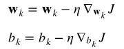
▌7. Softmax 回归算法
Softmax 回归算法,又称为多项式或多类别的 Logistic 回归算法。
给定:
Softmax 回归模型有以下几个特点:
训练 Softmax 回归模型有不同步骤。首先(在步骤0中),模型的参数将被初始化。在达到指定训练次数或参数收敛前,重复以下其他步骤。
第 0 步:用 0 (或小的随机值)来初始化权重向量和偏置值
第 1 步:对于每个类别k,计算其输入的特征与权重值的线性组合,也就是说为每个类别的训练样本计算一个得分值。对于类别k,输入向量为 ,则得分值的计算如下:
其中表示类别k的权重矩阵 ,·表示点积。
我们可以通过矢量化和矢量传播法则计算所有类别及其训练样本的得分值:

其中 X 是所有训练样本 的维度矩阵,W 表示每个类别的权重矩阵维度,其形式为
 ;
;
第 2 步:用 softmax 函数作为激活函数,将得分值转化为概率值形式。属于类别 k 的输入向量的概率值为:
同样地,我们可以通过矢量化来对所有类别同时处理,得到其概率输出。模型预测出的表示的是该类别的最高概率。
第 3 步:计算整个训练集的损失值。
我们希望模型预测出的高概率值是目标类别,而低概率值表示其他类别。这可以通过以下的交叉熵损失函数来实现:

在上面公式中,目标类别标签表示成独热编码形式( one-hot )。因此 为1时表示的目标类别是 k,反之则为 0。
第 4 步:对权重向量和偏置量,计算其对损失函数的梯度。
关于这个导数实现的详细解释,可以参见这里(http://ufldl.stanford.edu/tutorial/supervised/SoftmaxRegression/)。
一般形式如下:
对于偏置量的导数计算,此时为1。
第 5 步:对每个类别k,更新其权重和偏置值。
其中,表示学习率。
In [1]:
from sklearn.datasets import load_irisimport numpy as npfrom sklearn.model_selection import train_test_splitfrom sklearn.datasets import make_blobsimport matplotlib.pyplot as pltnp.random.seed(13)
数据集
In [2]:
X, y_true = make_blobs(centers=4, n_samples = 5000)fig = plt.figure(figsize=(8,6))plt.scatter(X[:,0], X[:,1], c=y_true)plt.title("Dataset")plt.xlabel("First feature")plt.ylabel("Second feature")plt.show()
In [3]:
# reshape targets to get column vector with shape (n_samples, 1)y_true = y_true[:, np.newaxis]# Split the data into a training and test setX_train, X_test, y_train, y_test = train_test_split(X, y_true)print(f'Shape X_train: {X_train.shape}')print(f'Shape y_train: {y_train.shape}')print(f'Shape X_test: {X_test.shape}')print(f'Shape y_test: {y_test.shape}')
Shape X_train: (3750, 2)
Shape y_train: (3750, 1)
Shape X_test: (1250, 2)
Shape y_test: (1250, 1)
Softmax回归分类
class SoftmaxRegressor: def __init__(self): pass def train(self, X, y_true, n_classes, n_iters=10, learning_rate=0.1): """ Trains a multinomial logistic regression model on given set of training data """ self.n_samples, n_features = X.shape self.n_classes = n_classes self.weights = np.random.rand(self.n_classes, n_features) self.bias = np.zeros((1, self.n_classes)) all_losses = [] for i in range(n_iters): scores = self.compute_scores(X) probs = self.softmax(scores) y_predict = np.argmax(probs, axis=1)[:, np.newaxis] y_one_hot = self.one_hot(y_true) loss = self.cross_entropy(y_one_hot, probs) all_losses.append(loss) dw = (1 / self.n_samples) * np.dot(X.T, (probs - y_one_hot)) db = (1 / self.n_samples) * np.sum(probs - y_one_hot, axis=0) self.weights = self.weights - learning_rate * dw.T self.bias = self.bias - learning_rate * db if i % 100 == 0: print(f'Iteration number: {i}, loss: {np.round(loss, 4)}') return self.weights, self.bias, all_losses def predict(self, X): """ Predict class labels for samples in X. Args: X: numpy array of shape (n_samples, n_features) Returns: numpy array of shape (n_samples, 1) with predicted classes """ scores = self.compute_scores(X) probs = self.softmax(scores) return np.argmax(probs, axis=1)[:, np.newaxis] def softmax(self, scores): """ Tranforms matrix of predicted scores to matrix of probabilities Args: scores: numpy array of shape (n_samples, n_classes) with unnormalized scores Returns: softmax: numpy array of shape (n_samples, n_classes) with probabilities """ exp = np.exp(scores) sum_exp = np.sum(np.exp(scores), axis=1, keepdims=True) softmax = exp / sum_exp return softmax def compute_scores(self, X): """ Computes class-scores for samples in X Args: X: numpy array of shape (n_samples, n_features) Returns: scores: numpy array of shape (n_samples, n_classes) """ return np.dot(X, self.weights.T) + self.bias def cross_entropy(self, y_true, scores): loss = - (1 / self.n_samples) * np.sum(y_true * np.log(scores)) return loss def one_hot(self, y): """ Tranforms vector y of labels to one-hot encoded matrix """ one_hot = np.zeros((self.n_samples, self.n_classes)) one_hot[np.arange(self.n_samples), y.T] = 1 return one_hot
初始化并训练模型
regressor = SoftmaxRegressor()w_trained, b_trained, loss = regressor.train(X_train, y_train, learning_rate=0.1, n_iters=800, n_classes=4)fig = plt.figure(figsize=(8,6))plt.plot(np.arange(800), loss)plt.title("Development of loss during training")plt.xlabel("Number of iterations")plt.ylabel("Loss")plt.show()Iteration number: 0, loss: 1.393
Iteration number: 100, loss: 0.2051
Iteration number: 200, loss: 0.1605
Iteration number: 300, loss: 0.1371
Iteration number: 400, loss: 0.121

数据分析咨询请扫描二维码


